5.9 KiB
Chapter 1 - Continuous Time Signals
Continuous Time Signal
A continuous time signal is a function x(t) that maps values from \Reals to \Reals or \Complex.
Causal Signals
A signal, x(t), is said to be causal if it has value 0 for t<0.
Non-causal Signals
A signal, x(t), is said to be non-causal, or not causal, if x(t) is not 0 for all t<0.
Finite Support
A signal, x(t), is said to have finite support, or finite duration, if there exists inputs T_1 and T_2 such that x(t) = 0 for t < T_1 and t > T_2.
Infinite Support
A signal, x(t), is said to have infinite support, or infinite duration, if it does not have infinite support.
There are three types of inifinite support:
- Right-sided: the signal has domain
(T_1, +\infty) - Left-sided: the signal has domain
(-\infty, T_2) - Two-sided: the signal has domain
(-\infty, +\infty)
1.1 Basic Signal Operations
Signal Addition
Signal addition is of the form: z(t) = x(t) + y(t), where the amplitude of the signal z(t) is the net amplitude of x(t) and y(t).
Scalar Multiplication
Scalar multiplication is of the form: z(t)=\alpha x(t). The amplitude of the output is proportional to \alpha.
Time Shift
A time shift is of the form: z(t)=x(t-\tau). When \tau > 0, the time shift is said to be a delay. When \tau < 0, the time shift is said to be an advance.
Time Scale
A time scale is of the form: z(t)=x(at). For \lvert a \rvert > 1, the scaling is said to be a compression. For \lvert a \rvert < 1, the scaling is said to be an expansion. For a < 0, a time reflection over t=0 occurs.
Figure 1.1.1 - Signal Transformations
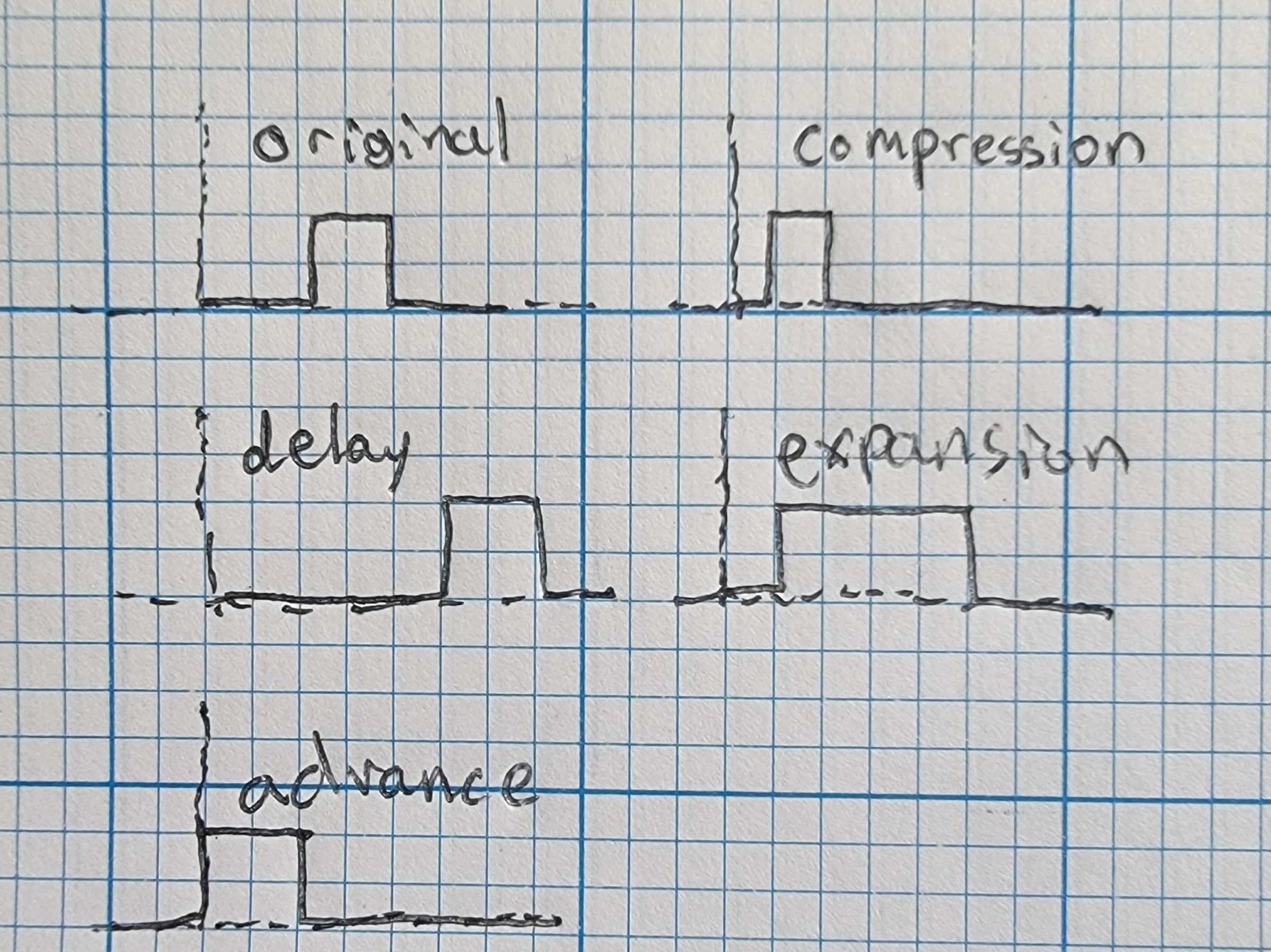
Figure 1.1.2 - Signal Combinations

1.2 Combinations of Operations
Review of Reflections
Every t becomes a -t.
x(t) = \begin{cases} t & 0 \leq t \leq 8 \\ 0 & otherwise \\ \end{cases}
Example 1
x(t) = \begin{cases} t & 0 \leq t \leq 8 \\ 0 & otherwise \\ \end{cases}
How to find y(t) = x(at - b)
Method 1 (recommended)
- Find
v(t) = x(t-b) - Find
w(t) = v(\lvert a \rvert t) = x( \lvert a \rvert t - b) - If
a \gt 0, then\lvert a \rvert = a.y(t) = w(t) = x(at - b) - If
a \lt 0, then\lvert a \rvert = a.y(t) = w(-t) = x(-\lvert a \rvert t - b)
Method 2
- Find
v(t) = x(\lvert a \rvert t) - Find
w(t) = v(t - \frac{b}{\lvert a \rvert}) = x(\lvert a \rvert \left(t - \frac{b}{\lvert a \rvert} \right))
Example
Find x(3t-5)
Lecture 5
The Impulse Function
\delta(t) = \begin{cases} 0 & t \ne 0 \\ \infty & t = 0 \\ \end{cases}
\int_{-\infty}^{\infty} \delta(t) dt = 1
\delta(t - \alpha) = \begin{cases} \infty & t=\alpha \\ 0 & t \ne \alpha \\ \end{cases}
\delta(2t - 3) = \begin{cases} \infty & 2t-3=0, t=3/2 \\ 0 & t \ne 3/2 \end{cases}
Properties
f(t) \delta(t- \alpha) = f(\alpha) \delta(t-\alpha)
\int_a^b f(t) \delta(t - \alpha)dt= \begin{cases} f(\alpha) & \alpha \in [a, b] \\ 0 & otherwise \end{cases}
Unit step
u(t) = \begin{cases} 1 & t \ge 0 \\ 0 & t \lt 0 \end{cases}
\delta(t) = \frac{du(t)}{dt}
u(t) = \int_{-\infty}^{t} \delta(\tau)d\tau = \begin{cases} 1 & t \ge 0 \\ 0 & t \lt 0 \end{cases}
u(t - \tau) = \begin{cases} 1 & t \ge \tau \\ 0 & t \lt \tau \end{cases}
u(-t + 5) = \begin{cases} 1 & t \le 5 \\ 0 & t \gt 5 \end{cases}
The difference between u(t) and u(t-1) is a finite support pulse from 0 to 1.
Ramp
r(t) = t u(t) = \begin{cases} t & t \ge 0 \\ 0 & t \lt 0 \end{cases}
\frac{dr(t)}{dt} = \frac{tdu(t)}{dt} + (1)u(t) = t\delta(t) + u(t) = u(t)
Derivatives
-
\cos(2 \pi t)\left[ u(t) - u(t-1) \right] = \begin{cases} 0 & t \lt 0 \\ \cos(2\pi t) & 0 \le t \lt 1 \\ 0 & t \ge 1 \end{cases}Using the product rule:
\cos(2\pi t)\left[ \delta(t) - \delta(t-1) \right] + -\sin(2\pi t)(2\pi)\left[u(t)-u(t-1)\right] -
u(t) - 2u(t-1) + u(t-2) = \begin{cases} 0 & t \lt 0 \\ 1 & 0 \le t \lt 1 \\ -1 & 1 \le t \lt 2 \\ 0 & t \ge 2 \end{cases}
Energy and Power of Signals
Energy
The energy of a signal x(t) could be finite or infinite.
Given a real or complex signal, x(t), the energy, E_x, is defined as:
E_x = \int_{-\infty}^{\infty} \lvert x(t) \rvert^2 dt-
If
x(t)has finite support, the domain is[a, b], and thereforeE_xis a finite integral with boundsaandb. -
If
x(t)has infinite support,E_xis an improper integral and may or may not have finite value. -
If
x(t)is periodic,E_xis infinite.
Power
The power, P_x, of an aperiodic signal is defined as:
P_x = \lim_{T \to \infty} \frac{1}{2T} \int_{-T}^{T} \lvert x(t) \rvert^2 dtThe power, P_x, of a periodic signal with period, T_0, x(t) is defined as:
P_x = \frac{1}{T_0}\int_{t_0}^{t_0 + T_0} \lvert x(t) \rvert^2 dtThe most convenient starting times, t_0 are -\frac{T_0}{2} and 0. The bounds of integration will be \left[ -\frac{T_0}{2}, \frac{T_0}{2} \right] and \left[ 0, T_0 \right] respectively.
For a periodic signal, the power is the energy of one period normalized by the length of the period.
FACT: A finite energy aperiodic signal has zero power.
P_x = \lim_{T \to \infty} \frac{1}{2T} \int_{-T}^{T} \lvert x(t) \rvert^2 dt=\lim_{T \to \infty} \frac{1}{2T} [N]Where N is some finite number.
\lim_{T \to \infty} \frac{N}{2T} = 0Procedure
- Determine if
x(t)is finite support or infinite support.- If finite support:
E_x \lt \infty,P_x = 0
- If finite support:
- If
x(t)is infinite support, determine periodicity ofx(t)- If aperiodic, calculate
E_x,P_x - If periodic:
E_x = \infty, calculateP_x
- If aperiodic, calculate
Facts
If:
x(t) = A\cos(\omega_0 t + \theta)Then:
E_x = \inftyP_x = \frac{A^2}{2}If:
x(t) = \sum_k A_k\cos(\omega_k t + \theta)Then:
E_x = \inftyP_x = \sum_k \frac{A_k^2}{2}