Rowan-Classes/5th-Semester-Fall-2023/Signals-and-Systems/Notes/Chapter2.md

Chapter 2 - Systems

A system, S, takes in an input signal, x(t), and outputs a signal, y(t).

x(t) \rightarrow \boxed{S} \rightarrow y(t)

y(t) = S[x(t)]

Simple System Properties

Linear Systems

S is said to be linear if it satisfies both hoogeneity and superposition.

Homogeneity

Scaling an input by a factor, a, scales the output by the same factor.

ay(t) = S[ax(t)]

Superposition

Adding two inputs lead to the corresponding outputs being added.

If

y_1(t) = S[x_1(t)]

y_2(t) = S[x_2(t)]

Then

y_1(t) + y_2(t) = S[x_1(t) + x_2(t)]

Time Invariance

S is said to be time-invariant if delaying or advancing the input gives the same delay or advance in the output.

y(t - \alpha) = S[x(t - \alpha)]

Causality

S is said to be causal if the output does not depend on any future inputs. Theoretically, noncausal systems cannot be realized.

Signal Boundedness

x(t) is said to be bounded if \lvert x(t) \rvert \le B_x \lt \infty

Bounded example:

x(t) = e^{-t} u(t)

Unbounded example:

x(t) = e^t u(t)

Bounded-Input, Bounded-Output Stability

S is said to be bounded-input, bounded-output (BIBO) stable if every bounded input gives rise to a bounded output.

Fact: The system is BIBO unstable if just one bounded input gives rise to an unbounded output.

Every bounded x(t) gives rise to a bounded y(t).

Example 2.1

y(t) = S[x(t)] = x^2(t)

Homogeneity:

S[ax(t)] = [ax(t)]^2 = a^2x^2(t)

ay(t) = ax^2(t)

Since S[ax(t)] \ne ay(t), S is not homogeneous, and therefore not linear.

Time invariance:

S[x(t-\alpha)] = [x(t-\alpha)]^2 = x^2(t-\alpha) =y(t-\alpha)

Since S[x(t-\alpha)] = y(t-\alpha), S is causal

BIBO stability:

\lvert x(t) \rvert \le B_x \lt \infty

\lvert y(t) \rvert = \lvert x^2(t) \rvert \le B_x^2 \lt \infty

Example 2.2

y(t) = S[x(t)] = \cos(x(t))

Homogeneity:

S[ax(t)] = \cos(ax(t))

ay(t) = a\cos(x(t))

Since S[ax(t)] \ne ay(t), S is not homogeneous and therefore not linear.

Time invariance:

S[x(t-\alpha)] = \cos(x(t-\alpha)) = y(t-\alpha)

BIBO stability:

\lvert x(t) \rvert \le B_x \lt \infty

\lvert y(t) \rvert \le 1

Example 2.3

y(t) = S[x(t)] = \lvert x(t) \rvert

Homogeneity:

S[ax(t)] = \lvert ax(t) \rvert

ay(t) = a \lvert x(t) \rvert

Since \lvert a \rvert \ne a, S is not homogeneous and therefore not linear.

Time invariance:

S[x(t-\alpha)] = \lvert x(t-\alpha)\rvert

y(t-\alpha) = \lvert x(t-\alpha)\rvert

Since S[x(t-\alpha)] = y(t-\alpha), S is time invariant.

BIBO stability

\lvert x(t) \rvert \le B_x \lt \infty

\lvert y(t) \rvert = \lvert x(t) \rvert \le B_x \lt \infty

Example 2.4

y(t) = S[x(t)] = mx(t) + b

Homogeneity:

S[ax(t)] = max(t) + b

ay(t) = amx(t) + ab

Superposition:

y_1(t) = mx_1(t) + b

y_2(t) = mx_2(t) + b

y_1(t) + y_2(t) = m(x_1(t) + x_2(t)) + 2b

For b=0, S is linear, otherwise, neither homogeneity nor superposition are satisfied.

Time invariance:

S[x(t-\alpha)] = mx(t-\alpha) + b

y(t-\alpha) = mx(t-\alpha) + b

Since y(t-\alpha) = x(t-\alpha), S is time invariant.

BIBO stability

\lvert y(t) \rvert = \lvert mx(t) + b \rvert \le \lvert m \rvert \lvert x(t) \rvert + \lvert b \rvert \le \lvert m \rvert B_x \lt \infty

Example 2.5

y(t) = S[x(t)] = tx(t+3)

Homogeneity:

S[ax(t)] = atx(t+3)

ay(t) = atx(t+3)

Superposition:

y_1(t) = tx_1(t+3)

y_2(t) = tx_2(t+3)

S[x_1(t) + x_2(t)] = t[x_1(t+3) + x_2(t+3)]

y_1 + y_2 = tx_1(t+3) + tx_2(t+3)

Since both homogeneity and superposition are satisfied, S is a linear system.

Time invariance:

S[x(t-\alpha)] = tx(t+3-\alpha)

y(t-\alpha) = (t-\alpha)\cdot x (t+3-\alpha)

Not time invariant.

Causality:

No

BIBO stability:

\lvert y(t) \rvert = \lvert tx(t+3) \rvert = \lvert t \rvert \lvert x(t+3)\rvert

Since \lvert t \rvert is not bounded, ther is no B_y such that:

\lvert y(t) \rvert \le B_y \lt \infty

Example 2.6 - Expansion

y(t) = S[x(t)] = x({t \over 10})

Homogeneity

S[ax(t)] = ax({t \over 10}) = ay(t)

Superposition

y_1(t) = x_1({t \over 10})

y_2(t) = x_2({t \over 10})

S[x_1(t) + x_2(t)] = x_1({t \over 10}) + x_2({t \over 10})

Time Invariance

S[x(t - \alpha)] = x({t \over 10} - \alpha)

y(t - \alpha) = x({t - \alpha \over 10})

Causal

y(-10) = x(-1)

BIBO Stability

Expansion affects input space, not output space

Example 2.7

y(t) = S[x(t)] = {1 \over T} \int\limits_{t-T}^t x(\tau)d\tau + B

Homogeneity

S[ax(t)] = {1 \over T} \int\limits_{t-T}^t ax(\tau)d\tau + B

ay(t) = {a \over T} \int\limits_{t-T}^t x(\tau)d\tau + B

Not homogeneous unless B = 0.

Superposition

y_1(t) = {1 \over T} \int\limits_{t-T}^t x_1(\tau)d\tau + B

y_2(t) = {1 \over T} \int\limits_{t-T}^t x_2(\tau)d\tau + B

S[x_1(t) + x_2(t)] = {1 \over T} \int\limits_{t-T}^t [x_1(\tau) + x_2(\tau)]d\tau + B

y_1(t) + y_2(t) = {1 \over T} \int\limits_{t-T}^t x_1(\tau)d\tau + {1 \over T} \int\limits_{t-T}^t x_2(\tau)d\tau + 2B

Time Invariance

S[x(t - \alpha)] = {1 \over T} \int\limits_{t-T}^t x(\tau - \alpha)d\tau + B

Substitute v = \tau - \alpha:

S[x(t - \alpha)] = {1 \over T} \int\limits_{t-T-\alpha}^{t-\alpha} x(v)dv + B

y(t - \alpha) = {1 \over T} \int\limits_{t-T-\alpha}^{t-\alpha} x(\tau)d\tau + B

Causality

y(t) depends on x(t) which uses inputs from t-T to t, and no future inputs. Therefore, the system is causal.

If instead, inputs ranged from t-T to t+T, the system would rely on future inputs and would not be causal.

BIBO Stability

\lvert x(t) \rvert \le B_x < \infty

|y(t)| = \left| {1 \over T} \int\limits_{t-T}^t x(\tau)d\tau + B \right|

|y(t)| \le \left| {1 \over T} \int\limits_{t-T}^t x(\tau)d\tau \right| + |B|

|y(t)| \le {1 \over T} \int\limits_{t-T}^t |x(\tau)|d\tau + |B|

|y(t)| \le {1 \over T} \int\limits_{t-T}^t B_x d\tau + |B|

|y(t)| \le {1 \over T} \left[\tau B_x\Big|_{t-T}^{t}\right] + |B|

|y(t)| \le {1 \over T} T B_x + |B|

|y(t)| \le B_x + |B|

Example 2.8 - AM

y(t) = S[m(t)] = m(t)\cos(\omega_c t)

Homogeneity

S[am(t)] = am(t)\cos(\omega_c t) ay(t)

Superposition

y_1(t) = m_1(t)\cos(\omega_c t)

y_2(t) = m_2(t)\cos(\omega_c t)

S[m_1(t) + m_2(t)] = [m_1(t) + m_2(t)]\cos(\omega_c t)

y_1(t) + y_2(t) = [m_1(t) + m_2(t)]\cos(\omega_c t)

Time Invariance

S[m(t-\alpha)] = m(t-\alpha)\cos(\omega_c t)

y(t - \alpha) = m(t-\alpha)\cos(\omega_c (t -\alpha))

Causality

Yes

BIBO Stability

|m(t)| \le B_x

|y(t)| = |m(t)\cos(\omega_c t)| \le |m(t)| \le B_x

Example 2.9 - FM

y(t) = S[m(t)] = \cos\left(\omega_c t + \int\limits_{-\infty}^{t} m(\tau) d\tau \right)

Homogeneity

S[am(t)] = \cos\left(\omega_c t + \int\limits_{-\infty}^{t} am(\tau) d\tau \right)

ay(t) = a\cos\left(\omega_c t + \int\limits_{-\infty}^{t} m(\tau) d\tau \right)

Time Invariance

S[m(t-\alpha)] = \cos\left(\omega_c t + \int\limits_{-\infty}^{t} m(\tau - \alpha) d\tau \right)

y(t-\alpha) = \cos\left(\omega_c (t - \alpha) + \int\limits_{-\infty}^{t} m(\tau) d\tau \right)

BIBO Stability

|y(t)| \le 1

Linear, Time-Invariant Systems

The implulse response h(t) of an LTI system is the output of the system when

\delta(t) \rightarrow \boxed{\text{LTI}} \rightarrow h(t)

Causal if h(t) = 0 for t<0.

BIBO stable if:

\int |h(t)|dt < \infty

If h(t) has finite supports, it is always BIBO stable. If h(t) has infinite support, BIBO stability must be checked.

A linear, constant coefficient ODE with input x(t) and output y(t) is LTI under zero initial conditions and when x(t) is a causal input.

Circuit Application

An RLC circuit with no initial voltage across the capacitor and no initial current through the inductor is LTI.

Without Initial Condition

For a capacitor with no initial voltage:

V(t) = S[I(t)] = {1\over C} \int\limits_0^t I(\tau) d\tau

Homogeneity

S[aI(t)] = {1\over C}\int\limits_0^t aI(\tau) d\tau = {a\over C}\int\limits_0^t I(\tau) d\tau = aV(t)

Superposition

V_1(t) = {1\over C}\int\limits_0^t I_1(\tau) d\tau

V_2(t) = {1\over C}\int\limits_0^t I_2(\tau) d\tau

S[I_1(t) + I_2(t)] = {1\over C} \int\limits_0^t [I_1(\tau) + I_2(\tau)]d\tau = V_1(t) + V_2(t)

Time Invariance

S[I(t - \alpha)] = {1\over C}\int\limits_{-\alpha}^{t-\alpha} I(\tau - \alpha) d\tau

S[I(t - \alpha)] = {1\over C}\int\limits_{-\alpha}^{t-\alpha} I(p) dp

If I(t) is causal:

S[I(t - \alpha)] = {1\over C}\int\limits_{0}^{t-\alpha} I(p) dp

V(t - \alpha) = {1\over C}\int\limits_0^{t-\alpha} I(\tau) d\tau

With Initial Condition

For a capacitor with initial voltage:

V(t) = {1\over C} \int\limits_0^t I(\tau) d\tau + V_0

Homogeneity

S[aI(t)] = {1\over C}\int\limits_0^t aI(\tau) d\tau + V_0

aV(t) = {a\over C}\int\limits_0^t I(\tau) d\tau + aV_0

Impulse Response

i(t) = \delta (t), h(t) = V(t) = ?

h(t) = {1 \over C} \int\limits_0^t \delta (\tau) d\tau = 
\begin{cases} 
{1\over C} & t \ge 0 \\
0 & t < 0
\end{cases}$$
$$h(t) = {1 \over C} u(t)$$

### Averager
$$y(t) = S[x(t)] = {1 \over T} \int\limits_{t-T}^t x(\tau) d\tau$$

#### Impulse response
$$h(t) = {1 \over T} \int\limits_{t-T}^t \delta(\tau) d\tau$$

3 possibilities for impulse response:
1. $0 < T - t$ means that the impulse is to the left of the limits of integration, and $h(t)$ is 0.
1. $T - t \le 0 \le t$ means that the impulse is within the bounds of integration, and $h(t)$ takes on a non-zero value.
1. $t > 0$ means that the impulse is to the right of the bounds of integration, nad $h(t)$ is 0.

For the second case, $T - t \le 0 \le t$, gives the response:
$$h(t) = \begin{cases}
{1 \over T} & 0 \le t \le T \\
0 & \text{elsewhere}
\end{cases} = {1\over T} \left[u(t) - u(t - T)\right]$$

Since $h(t)$ is 0 for $t < 0$, it is a causal signal.

## Convolution
$$y(t) = x(t)*h(t) = \int x(\tau) h(t - \tau)d\tau$$

##### Commutative:
$$x(t) * h(t) = \int h(\tau) x(t-\tau)d\tau = h(t) * x(t)$$

#### Case 1:
Two finite support wich have the same region of support (domain).
$$x(t) = h(t)$$

##### Step 1:
Decide to manipulate $x$ or $h$. 
$$h(t - \tau) = h(-\tau + t)$$
Since we are looking at $\tau$ as the variable, there is a reflection and an advance by $t$.

As $h(t-\tau)$ slides along the real number line, first there will be no overlap between $x(\tau)$ and $h(t - \tau)$. They multiply to 0, so $y(t) = 0$. Then, there will be some overlap, so $y(t)$ becomes:
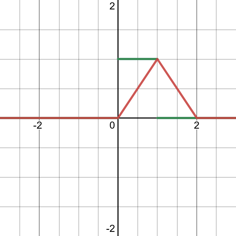
$$y(t) = \int\limits_0^t d\tau = t$$
$h(t-\tau)$ continues to slide and soon there is full overlap, so $y(t) = 1$.
![](Images/OverlapConvolution)